Lagrange Multipliers: Finding the Best Solution Under Constraints

What if you could find the best possible solution to a problem, even when the rules prevent you from choosing freely?

Imagine you have 10 metres of fencing and want to build a rectangular enclosure with the largest possible area.

You can choose the length and width. But you cannot make both arbitrarily large because the total perimeter must remain fixed.

How do you find the optimal dimensions?

You could test different rectangles. You could draw a graph. Or you could use a mathematical technique that finds the optimal solution directly.

That technique is called the method of Lagrange multipliers.

It is one of the most useful ideas in multivariable calculus because it connects geometry, derivatives, and optimization. The same principle appears in economics, physics, machine learning, engineering, and numerical optimization.

Let's understand how it works, why it works, and how to use it.

1. The Problem: Optimization Under Constraints

Optimization means finding the maximum or minimum value of a function.

For example, suppose we want to maximize a function:

$f(x,y)=xy$

If we can choose any values of (x) and (y), the function has no maximum: we can make (x) and (y) arbitrarily large.

But what if we impose a constraint?

$x+y=10$

Now we cannot choose (x) and (y) independently. If (x=3), then (y=7). If (x=6), then (y=4).

Our problem becomes:

$\text{Maximize } f(x,y)=xy$

subject to:

$g(x,y)=x+y-10=0$

The constraint limits the possible solutions to a line.

We want to find the point on that line where the product (xy) is greatest.

This is called constrained optimization.

Where does this appear in practice?

The same structure appears in many real problems:

Machine learning: Minimize a model's error while satisfying restrictions on its parameters.
Economics: Maximize utility while staying within a budget.
Engineering: Minimize material usage while meeting strength requirements.
Physics: Find equilibrium configurations subject to conservation laws.
Computer science: Optimize a system while respecting resource or capacity limits.

The details differ, but the mathematical structure is often remarkably similar.

2. First, Understand the Gradient

Before using Lagrange multipliers, we need to understand one important concept: the gradient.

For a function of two variables,

$f(x,y)$

the gradient is the vector of its partial derivatives:

$\nabla f= \begin{bmatrix} \frac{\partial f}{\partial x}\\[6pt] \frac{\partial f}{\partial y} \end{bmatrix}$

The gradient tells us the direction in which the function increases most rapidly.

For example, consider:

$f(x,y)=x^2+y^2$

Its partial derivatives are:

$\frac{\partial f}{\partial x}=2x$

$\frac{\partial f}{\partial y}=2y$

Therefore:

$\nabla f(x,y)= \begin{bmatrix} 2x\\ 2y \end{bmatrix}$

At the point ((1,2)), the gradient is:

$\nabla f(1,2)= \begin{bmatrix} 2\\ 4 \end{bmatrix}$

This vector points in the direction of the steepest increase of the function at that point.

You can think of the gradient as an arrow showing the uphill direction on a mathematical landscape.

What does the gradient have to do with optimization?

At an unconstrained local maximum or minimum of a differentiable function, the gradient is zero, provided the point is an interior point of the domain.

In other words:

$\nabla f=0$

But constrained optimization is different.

We cannot move in every direction. We must stay on the constraint.

That changes everything.

3. The Geometric Idea Behind Lagrange Multipliers

Return to our problem:

$\text{Maximize } f(x,y)=xy$

subject to:

$x+y=10$

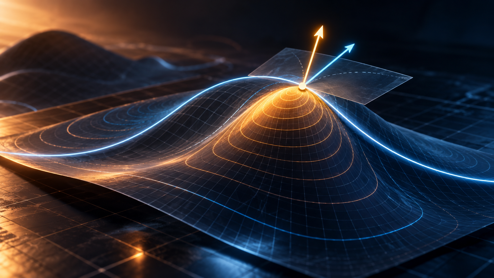
Imagine the constraint as a line drawn across a landscape representing the values of (f(x,y)).

We can move along the line, but we cannot leave it.

At the optimal point, moving along the constraint in either direction cannot increase the function to first order.

The gradient of the objective function must therefore be perpendicular to the constraint's tangent direction.

The gradient of the constraint is also perpendicular to that tangent direction.

Consequently, the two gradients must be parallel, provided the constraint is regular at the point.

Mathematically:

$\nabla f=\lambda\nabla g$

Here, (\lambda) is the Lagrange multiplier.

It is a scalar that tells us how the two gradients are related.

The crucial insight is that we do not necessarily need the gradient of the objective function to be zero.

Instead, it must align with the gradient of the constraint.

That is the central idea of the method.

4. The Lagrange Multiplier Formula

Suppose we want to optimize:

$f(x,y)$

subject to:

$g(x,y)=0$

We construct the Lagrangian function:

$\mathcal{L}(x,y,\lambda) = f(x,y)-\lambda g(x,y)$

Then we calculate its partial derivatives and set them equal to zero:

$\frac{\partial\mathcal{L}}{\partial x}=0$

$\frac{\partial\mathcal{L}}{\partial y}=0$

$\frac{\partial\mathcal{L}}{\partial\lambda}=0$

The last equation reproduces the original constraint:

$g(x,y)=0$

Equivalently, we solve the system:

$\nabla f=\lambda\nabla g$

$g(x,y)=0$

For a problem with two variables, this usually gives us three equations and three unknowns: (x), (y), and (\lambda).

For three variables, we have four unknowns: (x), (y), (z), and (\lambda).

The method generalizes naturally to higher dimensions.

Important: The equations give us candidate points. We still need to determine whether each candidate is a maximum, minimum, or neither.

5. Worked Example: Find the Maximum Product

Let's solve our original problem step by step.

We want to maximize:

$f(x,y)=xy$

subject to:

$x+y=10$

Step 1: Define the constraint

Write the constraint in the form (g(x,y)=0):

$g(x,y)=x+y-10$

Step 2: Calculate the gradients

For the objective function:

$f(x,y)=xy$

the gradient is:

$\nabla f= \begin{bmatrix} y\\ x \end{bmatrix}$

For the constraint:

$g(x,y)=x+y-10$

the gradient is:

$\nabla g= \begin{bmatrix} 1\\ 1 \end{bmatrix}$

Step 3: Apply the Lagrange multiplier condition

We use:

$\nabla f=\lambda\nabla g$

Substituting the gradients gives:

$\begin{bmatrix} y\\ x \end{bmatrix} = \lambda \begin{bmatrix} 1\\ 1 \end{bmatrix}$

This produces two equations:

$y=\lambda$

$x=\lambda$

Therefore:

$x=y$

This is already an interesting result.

The maximum occurs when the two variables are equal.

Step 4: Apply the constraint

We know that:

$x+y=10$

Since (x=y), we obtain:

$2x=10$

Therefore:

$x=5$

and:

$y=5$

Step 5: Calculate the function value

Substitute the coordinates into the original function:

$f(5,5)=5\cdot5$

Thus:

$\boxed{f_{\max}=25}$

The maximum product is 25, achieved at:

$\boxed{(x,y)=(5,5)}$

For nonnegative (x) and (y), this is the global maximum under the constraint (x+y=10).

We have found the optimal solution without testing every possible pair of numbers.

What does this mean geometrically?

The constraint is a straight line:

$x+y=10$

The objective function has level curves of the form:

$xy=c$

Each value of (c) corresponds to a different curve.

We are looking for the largest value of (c) for which the curve (xy=c) still intersects the constraint.

At the optimum, the two curves are tangent.

That tangency is the geometric reason the gradients become parallel.

6. A Second Example: The Shortest Distance to a Line

Now let's connect Lagrange multipliers to a problem you might encounter in university mathematics.

Find the minimum distance from the origin to the line:

$x+y=2$

The distance from a point ((x,y)) to the origin is:

$d=\sqrt{x^2+y^2}$

Instead of minimizing the square root, we can minimize its square:

$f(x,y)=x^2+y^2$

This gives the same minimizing point because the square root is strictly increasing for nonnegative values.

Our constraint is:

$g(x,y)=x+y-2=0$

Step 1: Calculate the gradients

The objective gradient is:

$\nabla f= \begin{bmatrix} 2x\\ 2y \end{bmatrix}$

The constraint gradient is:

$\nabla g= \begin{bmatrix} 1\\ 1 \end{bmatrix}$

Step 2: Apply the method

Using:

$\nabla f=\lambda\nabla g$

we obtain:

$2x=\lambda$

$2y=\lambda$

Therefore:

$x=y$

Step 3: Use the constraint

Since:

$x+y=2$

and (x=y), we get:

$2x=2$

Hence:

$x=1,\qquad y=1$

Step 4: Calculate the distance

The minimum squared distance is:

$d^2=1^2+1^2=2$

Therefore, the minimum distance is:

$\boxed{d_{\min}=\sqrt{2}}$

The closest point is:

$\boxed{(1,1)}$

Notice the connection to geometry: the vector from the origin to the closest point is perpendicular to the line.

Lagrange multipliers reveal that relationship algebraically.

Generalization to three dimensions

Suppose a plane is described by:

$Ax+By+Cz=D$

We want to find the point on the plane closest to the origin.

Minimize:

$f(x,y,z)=x^2+y^2+z^2$

subject to:

$g(x,y,z)=Ax+By+Cz-D=0$

The gradients are:

$\nabla f= \begin{bmatrix} 2x\\ 2y\\ 2z \end{bmatrix}$

and:

$\nabla g= \begin{bmatrix} A\\ B\\ C \end{bmatrix}$

The Lagrange equations give:

$2x=\lambda A$

$2y=\lambda B$

$2z=\lambda C$

This means the position vector of the closest point is parallel to the plane's normal vector.

Solving the equations gives the minimum distance:

$\boxed{ d_{\min}=\frac{|D|}{\sqrt{A^2+B^2+C^2}} }$

provided the plane is defined by a nonzero normal vector.

This formula is a beautiful example of how calculus can produce a general geometric result.

7. What Does the Lagrange Multiplier Actually Mean?

So far, (\lambda) has been an extra variable in our equations.

But it can have a useful interpretation.

Consider a more general constraint:

$g(x,y)=b$

We want to maximize or minimize (f(x,y)) while changing the value of (b).

Under suitable regularity and smoothness conditions, the Lagrange multiplier at an optimum can describe the rate at which the optimal objective value changes as the constraint value changes.

Using the convention:

$\mathcal{L}=f-\lambda(g-b)$

we obtain, under those conditions:

$\frac{d f^*}{db}=\lambda$

Here, (f^*) denotes the optimal value.

In practical terms, the multiplier can tell us how valuable a small relaxation of a constraint would be.

For example, imagine a factory maximizing production while limited by its available resources.

If the constraint represents the amount of a resource available, the corresponding multiplier may indicate how much the optimal production value would improve if the factory received a little more of that resource.

In economics and optimization, this is often called a shadow price.

The interpretation depends on the problem, the units, the sign convention, and whether the relevant regularity conditions hold.

8. Why Should Computer Science Students Care?

Lagrange multipliers are not just an exercise in calculus.

They help explain the mathematical structure behind many optimization problems.

Machine learning

Training a machine learning model often involves minimizing a loss function:

$\min_{\theta} L(\theta)$

Here, (\theta) represents the model parameters.

Some problems also impose constraints:

$g(\theta)=0$

or:

$h(\theta)\leq 0$

Lagrange multipliers provide a foundation for understanding how objective functions and constraints can be combined.

For inequality constraints, the broader framework is called the Karush–Kuhn–Tucker (KKT) conditions.

These conditions generalize the Lagrange multiplier approach and are important in constrained optimization.

Not every machine learning problem requires explicit Lagrange multipliers, but the underlying ideas appear throughout optimization theory.

Support vector machines

Support vector machines can be formulated as constrained optimization problems.

In the standard soft-margin formulation, the goal is to find a decision boundary while balancing classification errors against the size of the margin.

The dual formulation introduces Lagrange multipliers associated with the constraints.

These multipliers help determine which training examples influence the final decision boundary.

Those influential examples are known as support vectors.

Physics

In classical mechanics, constrained systems may have restrictions on their possible motion.

For example, a particle may be required to move along a surface rather than through unrestricted three-dimensional space.

Lagrange multipliers can be used to incorporate such constraints into equations of motion.

The corresponding multipliers can also be related to constraint forces, depending on the formulation.

The same mathematical idea therefore connects geometry, mechanics, and numerical optimization.

9. Common Mistakes to Avoid

When solving Lagrange multiplier problems, pay attention to the following details.

1. Forgetting the constraint equation

The Lagrange equations alone are not enough. Always include the original constraint.

2. Making sign errors

You may define the Lagrangian as:

$\mathcal{L}=f-\lambda g$

or:

$\mathcal{L}=f+\lambda g$

Both conventions are valid. They simply lead to different signs for the multiplier. Be consistent.

3. Assuming every candidate is a maximum

Solving the equations identifies stationary candidates, not automatically maxima or minima.

You must examine the candidates and the feasible region.

4. Ignoring boundary points

If the constraint defines a bounded curve or surface with endpoints or boundaries, those points may also need to be checked.

5. Forgetting regularity conditions

The standard method assumes the constraint gradient is nonzero at the candidate point:

$\nabla g\neq 0$

When this condition fails, the usual multiplier condition may not identify every constrained optimum.

6. Confusing a local optimum with a global optimum

A point can be locally optimal without being the best solution over the entire feasible set.

To establish a global result, additional reasoning may be necessary.

10. The General Method: A Practical Checklist

For a problem with an objective function (f(x,y)) and one equality constraint (g(x,y)=0), use this procedure:

Identify the objective. Decide what you need to maximize or minimize.
Write the constraint. Express it in the form (g(x,y)=0).
Calculate the gradients. Find (\nabla f) and (\nabla g).
Introduce the multiplier. Write (\nabla f=\lambda\nabla g).
Solve the system. Use the gradient equations together with the constraint.
Evaluate the candidates. Substitute each candidate into the original objective.
Check the conditions. Consider boundaries, regularity, and whether the result is local or global.

For multiple equality constraints, introduce one multiplier for each constraint.

The method is systematic, but the reasoning behind it is geometric.

You are searching for a point where the objective cannot improve through a small movement that respects the constraints.

11. Test Your Understanding

Try solving these problems before looking at the solutions.

Problem 1: Maximum product

Find the maximum of:

$f(x,y)=xy$

subject to:

$x+y=12$

Assume (x,y\geq 0).

Questions:

What are the gradients?
What equations do you obtain from the Lagrange multiplier condition?
What is the maximum value?

The gradients are:

$\nabla f= \begin{bmatrix} y\\ x \end{bmatrix}, \qquad \nabla g= \begin{bmatrix} 1\\ 1 \end{bmatrix}$

The Lagrange equations give:

$y=\lambda,\qquad x=\lambda$

Therefore:

$x=y$

Using (x+y=12):

$x=y=6$

The maximum is:

$\boxed{f_{\max}=36}$

Problem 2: Minimum distance

Find the point on the line:

$2x+y=6$

that is closest to the origin.

Minimize:

$f(x,y)=x^2+y^2$

subject to:

$g(x,y)=2x+y-6=0$

The gradients are:

$\nabla f= \begin{bmatrix} 2x\\ 2y \end{bmatrix}, \qquad \nabla g= \begin{bmatrix} 2\\ 1 \end{bmatrix}$

The Lagrange equations are:

$2x=2\lambda$

$2y=\lambda$

Thus:

$x=\lambda,\qquad y=\frac{\lambda}{2}$

Substitute into the constraint:

$2\lambda+\frac{\lambda}{2}=6$

$\frac{5\lambda}{2}=6$

Therefore:

$\lambda=\frac{12}{5}$

The closest point is:

$\boxed{\left(\frac{12}{5},\frac{6}{5}\right)}$

The minimum distance is:

$d_{\min} = \sqrt{\left(\frac{12}{5}\right)^2+ \left(\frac{6}{5}\right)^2}$

Therefore:

$\boxed{d_{\min}=\frac{6}{\sqrt{5}}}$

Final Thought

Lagrange multipliers are a reminder that optimization is not always about finding the steepest path uphill or downhill.

Sometimes, the possible directions are restricted.

The key is to find the point where the objective function can no longer improve while respecting those restrictions.

Once you understand why the gradients become parallel, the equations stop looking like an arbitrary recipe. They become a direct expression of the geometry of the problem.

Learn the geometry, understand the equations, and the method becomes much easier to remember.